The Lagrangian Approach to Solving Mechanical Systems
In a previous article, I discussed a few basic concepts regarding the Lagrangian approach to classical mechanics, including constraints, generalized coordinates, virtual work, etc. Further, I also listed some limitations that make the Newtonian approach sorely incompetent for systems that deviate even the slightest bit from highly idealized and simplistic scenarios.
Today, we will take a quick glance at the Lagrangian approach to solving problems in classical mechanics by solving a familiar problem: that of the simple pendulum. My argument for this is that once you are through with the solution, you will be able to appreciate just how superior the Lagrangian approach is. However, as we will see, all’s not well even if it does end well with the Lagrangian approach. Let’s get started.
What is the Lagrangian?
Before I define this quantity, here is a quick distinction between the mechanics you study in the beginning and the Lagrangian approach. If you think about it, you will notice how all problems in Newtonian mechanics were concerned with forces, which is precisely where trouble began to brew.
On the other hand, the Lagrangian approach utilizes energy as the “primary” quantity, per se. The central quantity while tackling problems via this approach is a function known as the Lagrangian. It can summarize the entire dynamics of a system and can take on various forms. While I cannot list the Lagrangian for all possible systems here, I can nonetheless give you an expression that is valid for non-relativistic systems, which is as follows
L = T — V
Here, T is the kinetic energy of the system, and V is its potential energy.
So How Does That Help Us?
In more ways than one, as it turns out. While the exact derivation is beyond and not the scope of this article, it can be shown that for systems where the potential is independent of generalized velocities, the following equations are satisfied:

And yes, the use of the plural “equations” was intentional, for the above image is not a single equation. Instead, it corresponds to a set of equations, each managing the derivatives of the Lagrangian with one particular pair of generalized coordinate and velocity. Thus, if you had a system with three generalized coordinates, you would need to solve three such equations before arriving at a solution for the system. You will see what I mean as we tackle our example problem.
The Simple Pendulum
While the simple pendulum is well-known to all, I still state the problem here formally for the sake of recall:
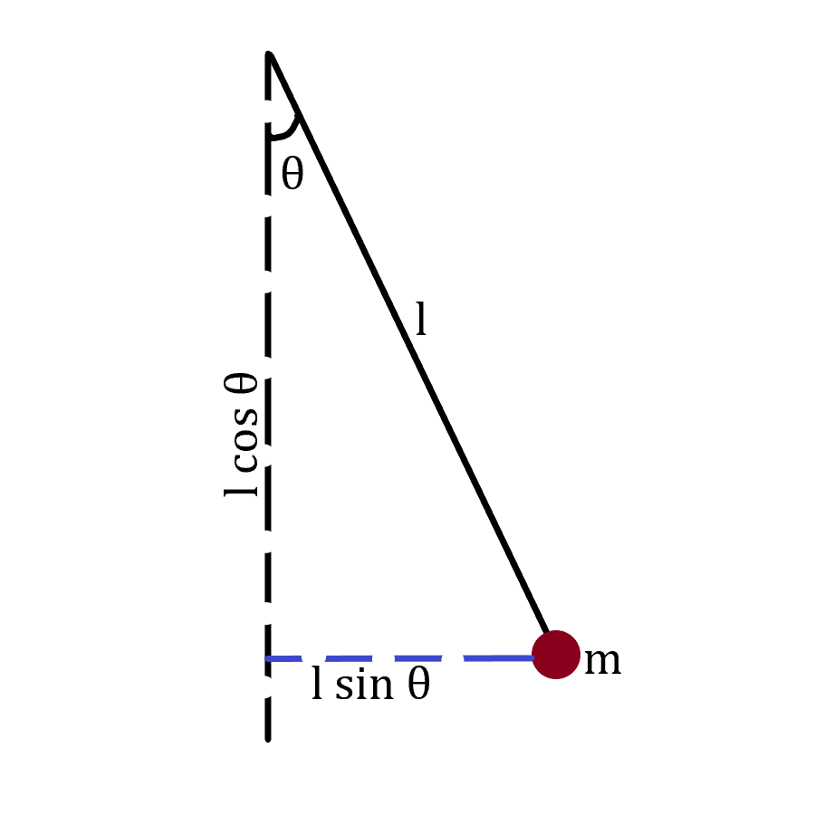
A bob of mass m hangs from a massless string affixed to a point O that is stationary. If the string remains taut at all times, describe the motion of the system, assuming that the angle made by the string with the vertical is very small.
1. The generalized coordinates
A student acquainted with the Cartesian system would be inclined to use the same for tackling this approach. However, let’s shift our perspective and look at the angle made by the string with the vertical, calling it θ in the process. In such a case, we can write the x and y coordinates of the pendulum as follows:

Do you see how these equations help us? If not, recall our discussion about generalized coordinates from the previous article linked in the beginning of this one. With these equations, we can find our generalized coordinates which, with x and y depending on θ, comes out to be θ and thus, we can use the latter to completely describe the motion of our system.
2. The Lagrangian
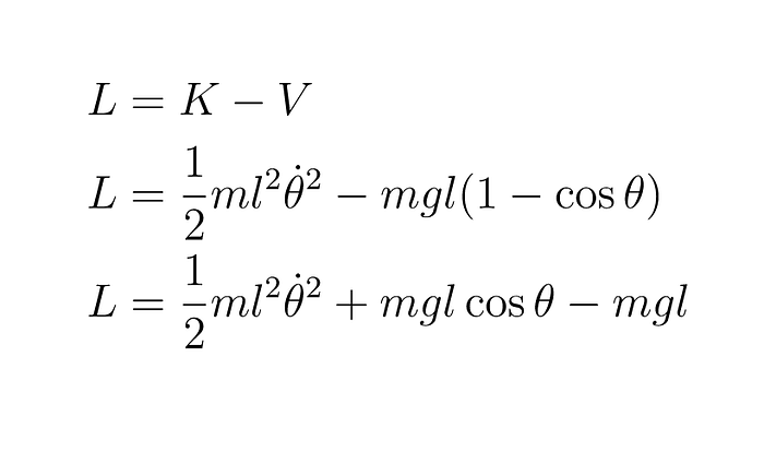
Expressing the Lagrangian is now quite trivial, albeit slightly confusing if one is inexperienced. The confusion arises since it involves a potential term, which varies depending on the reference point you have taken. Personally, I find taking the point at which the bob hangs vertically as the zero to be the most suitable as the “zero-point”. This way, whenever the pendulum swings away, it gains potential energy, whilst simultaneously losing kinetic energy.
Thus, the potential energy when the pendulum makes an angle θ with the vertical is V = mg × height of bob above the zero point. That is,
V = mg l (1- cos θ).
And the kinetic energy may be written as follows:
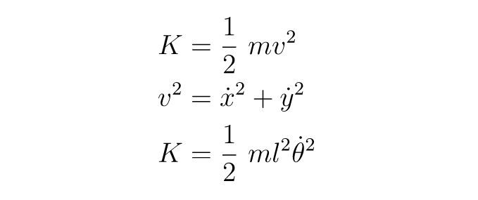
From the above expressions, you can easily find the Lagrangian of the system, and we are one step closer to our solution.
3. Solving the Euler-Lagrange Equations
Recall how I mentioned that the Euler-Lagrange equations are plural. You solve not one, but as many as the number of generalized coordinates in the system. While this keeps you safe from second-order equations, it can add significantly to the complexity if there are too many generalized coordinates. But I digress.
For the case of the simple pendulum, there is only one generalized coordinate, and that is θ. Let us state the Lagrangian of the system in terms of this variable.
Next, we plug this value into the Euler-Lagrange equation, noting that q ≡ θ. Thus,

Notice how the additional term of -mgl in the Lagrangian didn’t make a difference since it went to zero upon being differentiated; just a small reminder to trust the process.
Now, what we have derived above is indeed our answer. But does this equation feel a tad unfamiliar to you? It should, because so far, we haven’t applied the small-angle approximation as stated in our problem. Recall that
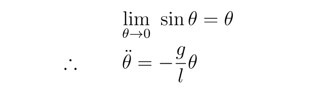
And there we have it, the official solution to the simple pendulum problem, arrived at using Lagrangian mechanics instead of Newtonian concepts.
Conclusion
From the above exercise, I hope you have developed a suitable understanding of how to tackle a problem via the Lagrangian approach. I would suggest that you try and solve the following problems to develop a better appreciation:
- The double pendulum: Two simple pendulums, with pendulum number two hanging from the bob of the first pendulum.
- Pendulum and block: A block is placed on a frictionless floor and attached to the end of a massless spring. From the block also hangs a simple pendulum. Try and find the equations of motion of both the objects.
The Lagrangian approach might feel a bit convoluted when you use it for problems you are already familiar with, but as soon as systems start to deviate from the simplicity you are acquainted with, you will realize how much easier this approach becomes.
The ease in the Lagrangian arises out of a set of factors, two of which are:
- A reduced number of variables to work with. And,
- First order equations instead of second order ones.
At the same time, Lagrangian approach requires solving a larger number of equations and thus, it is a mixed bag here. Nevertheless, in certain situations, it can come in pretty handy.